Tutorials
This page contains a range of tutorials explaining installation, setup, usage and example output to help you get started with TomoBEAR.
First of all, you have to setup TomoBEAR:
-
Video-tutorial explaining how to get the latest
TomoBEARversion and configureTomoBEARand its dependencies.
To provide an example of the TomoBEAR processing project we have chosen the well-known cryo-ET benchmarking data set containing 80S ribosomes - EMPIAR-10064.
In this tutorial we will:
- explain structure and important parameters of the input
JSONfile used as a configuration file inTomoBEARprojects; - explain output data structure of
TomoBEARprojects; - explain pipeline execution and control by checkpoint files;
- guide you through the processing of the famous real-world dataset EMPIAR-10064 to achieve resolution of 11.3 Å with 4003 particles in nearly-automated parallelized manner.
We have prepared a range of short (8-12 min) video-tutorials following the written version of the 80S ribosome tutorial provided below:
- Video-tutoral 1: description of the project configuration file and the pipeline execution
-
Video-tutoral 2: additional configuration file parameters description,
TomoBEAR-IMOD-TomoBEARloop for checking tilt series alignment results and fiducials refinement (if needed); - Video-tutoral 3: checking on further intermediate results (alignment, CTF-correction, reconstruction, template matching).
You can download EMPIAR-10064 data set here (mixedCTEM part): https://www.ebi.ac.uk/empiar/EMPIAR-10064. After downloading the data extract it in a folder of your choice.
In our case we used just the mixedCTEM data and achieved 11.3 Å in resolution with 4003 particles which is similar to the resolution achieved by the original researchers. If you want you can additionally use the CTEM data to be able to pick even more particles.
In the TomoBEAR source code folder you will find a subfolder configurations/ containing a file ribosome_empiar_10064_dynamo.json. This file describes the processing pipeline which should be setup by TomoBEAR to process used in this tutorial data set.
The whole JSON file used for this tutorial you may also find at the end of this tutorial.
The following paragraphs will explain the variables contained in the JSON file and the needed changes to be able to run TomoBEAR on your local machine.
First of all and most importantly you need to show TomoBEAR the path to the data and the processing folder. This must be done in the section "general": {} of the JSON file, as shown below:
    "general": {
        "project_name": "Ribosome",
        "project_description": "Ribosome EMPIAR 10064",
        "data_path": "/path/to/ribosome/data/*.mrc",
        "processing_path": "/path/to/processing/folder",
        "expected_symmetrie": "C1",
        "apix": 2.62,
        "tilt_angles": [-60.0, -58.0, -56.0, -54.0, -52.0, -50.0, -48.0, -46.0, -44.0, -42.0, -40.0, -38.0, -36.0, -34.0, -32.0, -30.0, -28.0, -26.0, -24.0, -22.0, -20.0, -18.0, -16.0, -14.0, -12.0, -10.0, -8.0, -6.0, -4.0, -2.0, 0.0, 2.0, 4.0, 6.0, 8.0, 10.0, 12.0, 14.0, 16.0, 18.0, 20.0, 22.0, 24.0, 26.0, 28.0, 30.0, 32.0, 34.0, 36.0, 38.0, 40.0, 42.0, 44.0, 46.0, 48.0, 50.0, 52.0, 54.0, 56.0],
        "rotation_tilt_axis":-5,
        "gold_bead_size_in_nm": 9,
        "template_matching_binning": 8,
        "binnings": [2, 4, 8],
        "reconstruction_thickness": 1400,
        "as_boxes": false
  }
Since the pixel size and tilt angles are not provided in the header of MRC files of the used here data set EMPIAR-10064, we have to add this information in the "general": {} section of the configuration file.
Everything else should be fine for now and the processing can be started. To run the TomoBEAR on the ribosome data set you need to type in the following command in the command window of MATLAB
runTomoBear("local", "/path/to/ribosome_empiar_10064_dynamo.json")or if you are using a compiled version of TomoBEAR and have everything set up properly type in the following command on the command line from the TomoBEAR folder
./run_tomoBEAR local /path/to/ribosome_empiar_10064_dynamo.json /path/to/defaults.jsonWhen you followed all the steps thoroughly TomoBEAR should run up to the first appearence of StopPipeline. That means the following modules will be executed.
    "MetaData": {
    },
    "CreateStacks": {
    },
    "DynamoTiltSeriesAlignment": {
    },
    "DynamoCleanStacks": {
    },
    "BatchRunTomo": {
        "skip_steps": [4],
        "ending_step": 6
    },
    "StopPipeline": {
    },
This can take a while, as the result of this segment TomoBEAR will create a folder structure with subfolders for the individual steps. You can monitor the progress of the execution in shell and by inspecting the contents of the folders. Upon success of an operation a file SUCCESS is written inside each folder. If you want to rerun a step you can terminate the process, change parameters, remove the SUCCESS file (or the entire subfolder) and restart the process.
Here the stacks have already been assembled, so neither "Motioncor2": {}, nor "SortFiles": {} modules were not needed. Here the key functionality is performed by "DynamoTiltSeriesAlignment": {} (a recommended tutorial) after which the projections containing low number of tracked gold beads are excluded by "DynamoCleanStacks": {}. Finally, the output is converted into an IMOD project. The running time depends on your infrastructure and setup.
After TomoBEAR stops you can inspect the fiducial model in the folder of "BatchRunTomo": {} which you can find in your processing folder.
cd /path/to/your/processing/folder/5_BatchRunTomo_1Now you can inspect the alignment of every tilt stack one after the other and can possibly refine it if needed. For that you can use the following command. Please replace xxx with the tomogram number(s) that you want to inspect.
etomo tomogram_xxx/*.edfWhen etomo starts just chose the fine alignment step which should be magenta-colored if everything went fine for that tomogram and then click on edit/view fiducial model to start 3dmod with the right options to be able to refine the gold beads. If you do not see the green circles - please go to the IMODimod command window, Edit -> Object l-> Type-> activate scattered and increase the size of the circle to e.g. 5.
Before you start to refine just press the arrow up button in the top left corner of the window with the view port in order to zoom in. To refine the gold beads click on Go to next big residual in the window with the stacked buttons from top to bottom and the view in the view port window should change immediately to the location of a gold bead with a big residual.
Now see if you can center the marker better on the gold bead with the right mouse button. It is important that you don't put it on the peak of the red arrow but center it on the gold bead. When you are finished with this gold bead just press again on the Go to next big residual button. After you are finished with re-centering the marker on the gold beads you need to press the Save and run tiltalign button.
After you finished the inspection of all the alignments you can start TomoBEAR again as previously and it will continue from where it stopped up to the next StopPipeline section.
To continue running TomoBEAR on the Ribosome data set you need to type in as previously the following command in the command window of MATLAB
runTomoBear("local", "/path/to/ribosome_empiar_10064_dynamo.json")or if you are using a compiled version of TomoBEAR and have everything set up properly type in the following command on the command line from the TomoBEAR folder
./run_tomoBEAR local /path/to/ribosome_empiar_10064_dynamo.json /path/to/defaults.jsonTomoBEAR should now detect that it has stopped at the previous step StopPipeline and continue from where it stopped. The following excerpt from the ribosome_empiar_10064_dynamo.json file is describing what TomoBEAR needs to do next.
    "BatchRunTomo": {
        "starting_step": 8,
        "ending_step": 8
    },
    "GCTFCtfphaseflipCTFCorrection": {
    },
    "BatchRunTomo": {
        "starting_step": 10,
        "ending_step": 13
    },
    "BinStacks": {
    },
    "Reconstruct": {
    },
    "DynamoImportTomograms": {
    },
    "EMDTemplateGeneration": {
        "template_emd_number": "3420",
        "flip_handedness": true
    },
    "DynamoTemplateMatching": {
        "sampling": 15,
        "size_of_chunk": [463, 463, 175]
    },
    "TemplateMatchingPostProcessing": {
        "cc_std": 2.5
    },
This segment performs estimation of defocus, and hence, of the Contrast Transfer Function (CTF) using GCTF and subsequent CTF-correction using Ctfphaseflip from IMOD ("GCTFCtfphaseflipCTFCorrection": {}). You can inspect the quality of fitting by going into the folder 8_GCTFCtfphaseflipCTFCorrection_1 and typing imod tomogram_xxx/slices/*.ctf and making sure that the Thon rings match the estimation. If not - play with the parameters of the GCTFCtfphaseflipCTFCorrection module.
Then binned aligned CTF-corrected stacks are produced by "BinStacks": {} and tomographic reconstructions are generated for the binnings specified in the section "general": {}. In this example the particles are picked using template matching. First a template from EMDB is produced at a proper voxel size, then "DynamoTemplateMatching": {} creates cross-correlation (CC) volumes which can be inspected.
Note
At a high binning level (e.g. 8 or 16) using the whole volume as a single chunk is more optimal than doing several chunks, so it is important to set the corresponding parameter to the size of the binned tomogram used for template matching.
Finally, highest cross-correlation peaks, over 2.5 standard deviations above the mean value in the cross-correlation volume are selected for extraction to 3D particle files, the initial coordinates are stored in the particles_table folder as a file in the dynamo table format.
In the section below you will find subtomogram classification projects that should produce you a reasonable structure. They first use multi-reference alignment projects with a true class and so-called noise trap classes to first classify out false-positive particles produced by template matching, this happens at the binning which was used for template matching. In the end of the segment you should have a reasonable set of particles in the best class.
    "DynamoAlignmentProject": {
        "iterations": 3,
        "classes": 4,
        "use_noise_classes": true,
        "use_symmetrie": false
    },
    "DynamoAlignmentProject": {
        "iterations": 3,
        "classes": 4,
        "use_noise_classes": true,
        "use_symmetrie": false,
        "selected_classes": [1]
    },
    "DynamoAlignmentProject": {
        "iterations": 3,
        "classes": 4,
        "use_noise_classes": true,
        "use_symmetrie": false,
        "selected_classes": [1]
    },
    "DynamoAlignmentProject": {
        "iterations": 3,
        "classes": 4,
        "use_noise_classes": true,
        "use_symmetrie": false,
        "selected_classes": [1]
    },
    "DynamoAlignmentProject": {
        "iterations": 3,
        "classes": 4,
        "use_noise_classes": true,
        "use_symmetrie": false,
        "selected_classes": [1]
    },
    "DynamoAlignmentProject": {
        "iterations": 3,
        "classes": 4,
        "use_noise_classes": true,
        "use_symmetrie": false,
        "selected_classes": [1]
    },
    "DynamoAlignmentProject": {
        "iterations": 3,
        "classes": 3,
        "use_noise_classes": true,
        "use_symmetrie": false,
        "selected_classes": [1],
        "box_size": 1.10,
        "binning": 4
    },
    "StopPipeline": {
    },
After subtomogram classification projects done, you should have a reasonable set of particles in the best class which you should select. To select the best class you need to go into the last DynamoAlignmentProject folder before the last produced StopPipeline folder, and then go to alignment_project_1_bin_y/mraProject_bin_y/results/iteQQQQ/averages (where iteQQQQ corresponds to the pre-last iteration folder) and type imod average_ref_CCC_ite_QQQQ.em to open produced average for each class CCC to identify the best class to use further.
Variables binning y, pre-last iteration number QQQQ and class numbers CCC can depend on parameters used in DynamoAlignmentProject. But if you repeat instructions provided in this tutorial, this should be the folder 23_DynamoAlignmentProject_1/alignment_project_1_bin_4/mraProject_bin_4/results/ite0012/averages where you may find files average_ref_001_ite_0012.em, average_ref_002_ite_0012.em, and average_ref_003_ite_0012.em corresponding to the produced averages for 3 classes, from which you should choose the best one.
Once you have selected the best class, insert corresponding class number in the list [] as a value of the parameter "selected_classes" to the following section to be executed by TomoBEAR:
    "DynamoAlignmentProject": {
        "classes": 1,
        "iterations": 1,
        "use_noise_classes": false,
        "swap_particles": false,
        "use_symmetrie": false,
        "selected_classes": [3],
        "binning": 4,
        "threshold":0.8
    },
The section above is called single reference project, which will split the particles of the previously selected best class into two equally sized classes (called even/odd halves) with subsequent alignment of the particles in those halves to produce corresponding averages. This division will be needed further when unbinned data will be produced to be able to calculate the resolution of the resulting averaged map using Fourier Shell Correlation (FSC) curve.
After the first single reference project introduced above you will need to process tomograms by similar projects but at lower binnings in order to reduce the voxel size up to unbinned data to get the information corresponding to the highest possible resolution to be achieved using the current data set. At this point automated workflow is finished as the user needs to play with the masks, particle sets, etc.
You may want to try to use the following example of the end section of JSON file in order to have experience of processing tomograms at lower binnings to produce unbinned data to finally be able to calculate resolution of your ribosome electron-density map as a result of the first experience with TomoBEAR!
    "DynamoAlignmentProject": {
        "classes": 1,
        "iterations": 1,
        "use_noise_classes": false,
        "swap_particles": false,
        "use_symmetrie": false,
        "selected_classes": [1,2],
        "binning": 2,
        "threshold":0.9
    },
    "BinStacks":{
        "binnings": [1],
        "use_ctf_corrected_aligned_stack": false,
        "use_aligned_stack": true,
        "run_ctf_phaseflip": true
    },
    "Reconstruct": {
        "reconstruct": "unbinned"
    },
    "DynamoAlignmentProject": {
        "classes": 1,
        "iterations": 1,
        "use_noise_classes": false,
        "swap_particles": false,
        "use_symmetrie": false,
        "selected_classes": [1,2],
        "binning": 1,
        "threshold":1
    }
Consider, that after performing first single reference project you need to select both halves from the previous step by setting "selected_classes": [1,2] (in order to keep all particles) while producing one class by setting "classes": 1 at the subsequent steps of binning reduction using "DynamoAlignmentProject": {} module.
If you get out of memory error while running some of "DynamoAlignmentProject": {} at lower binnings (especially the last one), you may put additional parameter "dt_crop_in_memory": 0 to the corresponding "DynamoAlignmentProject": {} sections in order to prevent keeping the whole tomogram in memory for processing. For example, in this tutorial size of the one of unbinned tomograms is ~72Gb, while for binning 2 it is near 9Gb.
Finally, to estimate resolution of produced by TomoBEAR results, you need to use the following Dynamo command in MATLAB:
fsc = dfsc(path_to_half1, path_to_half2, 'apix', 2.62, 'mask', path_to_mask, 'show', 'on')
where path_to_half1 and path_to_half2 are paths to the prelast iteration results of the last DynamoAlignmentProject folder, which in this tutorial are located in 29_DynamoAlignmentProject_1/alignment_project_1_bin_1/mraProject_bin_1_eo/results/ite0006/averages, where you may find files average_ref_001_ite_0006.em and average_ref_002_ite_0006.em corresponding to the averages made from halves of the resulting particles set.
You also need to use a mask to filter averages for FSC calculation, and the accuracy of the used mask have impact on the resolution estimation. Appropriate mask to use for the initial resolution estimation you may find in the last DynamoAlignmentProject folder in a file called mask.em (in this tutorial path_to_mask is 29_DynamoAlignmentProject_1/mask.em).
After that you should get a similar FSC curve to the following one:
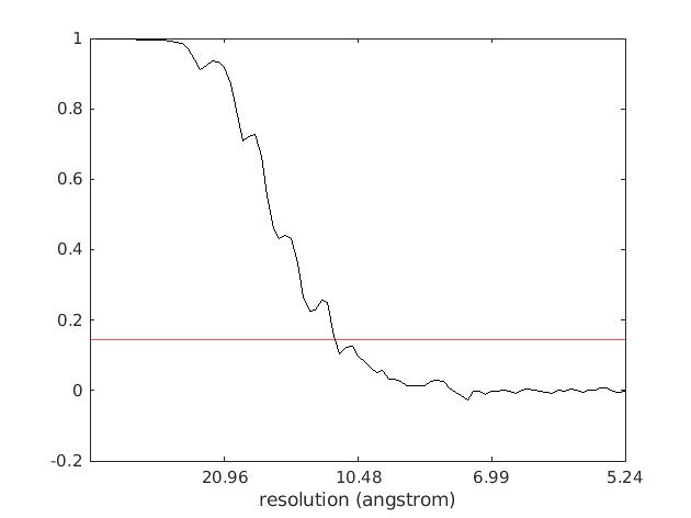
where in red we added a so-called "gold-standard" criterion of FSC = 0.143 to estimate the final map resolution, which in our case for the final set of ~4k ribosome particles reached 11.3Å.
Here the Ribosome data set-based tutorial is finished. We thank you for trying out TomoBEAR and hope you have enjoyed it!
The full `JSON` configuration file to setup the processing pipeline and data in `TomoBEAR` (expand to see)
{
    "general": {
        "project_name": "Ribosome",
        "project_description": "Ribosome EMPIAR 10064",
        "data_path": "/path/to/ribosome/data/*.mrc",
        "processing_path": "/path/to/processing/folder",
        "expected_symmetrie": "C1",
        "apix": 2.62,
        "tilt_angles": [-60.0, -58.0, -56.0, -54.0, -52.0, -50.0, -48.0, -46.0, -44.0, -42.0, -40.0, -38.0, -36.0, -34.0, -32.0, -30.0, -28.0, -26.0, -24.0, -22.0, -20.0, -18.0, -16.0, -14.0, -12.0, -10.0, -8.0, -6.0, -4.0, -2.0, 0.0, 2.0, 4.0, 6.0, 8.0, 10.0, 12.0, 14.0, 16.0, 18.0, 20.0, 22.0, 24.0, 26.0, 28.0, 30.0, 32.0, 34.0, 36.0, 38.0, 40.0, 42.0, 44.0, 46.0, 48.0, 50.0, 52.0, 54.0, 56.0],
        "rotation_tilt_axis":-5,
        "gold_bead_size_in_nm": 9,
        "template_matching_binning": 8,
        "binnings": [2, 4, 8],
        "reconstruction_thickness": 1400,
        "as_boxes": false
    },
    "MetaData": {
    },
    "CreateStacks": {
    },
    "DynamoTiltSeriesAlignment": {
    },
    "DynamoCleanStacks": {
    },
    "BatchRunTomo": {
        "skip_steps": [4],
        "ending_step": 6
    },
    "StopPipeline": {
    },
    "BatchRunTomo": {
        "starting_step": 8,
        "ending_step": 8
    },
    "GCTFCtfphaseflipCTFCorrection": {
    },
    "BatchRunTomo": {
        "starting_step": 10,
        "ending_step": 13
    },
    "BinStacks": {
    },
    "Reconstruct": {
    },
    "DynamoImportTomograms": {
    },
    "EMDTemplateGeneration": {
        "template_emd_number": "3420",
        "flip_handedness": true
    },
    "DynamoTemplateMatching": {
        "sampling": 15,
        "size_of_chunk": [463, 463, 175]
    },
    "TemplateMatchingPostProcessing": {
        "cc_std": 2.5
    },
    "DynamoAlignmentProject": {
        "iterations": 3,
        "classes": 4,
        "use_noise_classes": true,
        "use_symmetrie": false
    },
    "DynamoAlignmentProject": {
        "iterations": 3,
        "classes": 4,
        "use_noise_classes": true,
        "use_symmetrie": false,
        "selected_classes": [1]
    },
    "DynamoAlignmentProject": {
        "iterations": 3,
        "classes": 4,
        "use_noise_classes": true,
        "use_symmetrie": false,
        "selected_classes": [1]
    },
    "DynamoAlignmentProject": {
        "iterations": 3,
        "classes": 4,
        "use_noise_classes": true,
        "use_symmetrie": false,
        "selected_classes": [1]
    },
    "DynamoAlignmentProject": {
        "iterations": 3,
        "classes": 4,
        "use_noise_classes": true,
        "use_symmetrie": false,
        "selected_classes": [1]
    },
    "DynamoAlignmentProject": {
        "iterations": 3,
        "classes": 4,
        "use_noise_classes": true,
        "use_symmetrie": false,
        "selected_classes": [1]
    },
    "DynamoAlignmentProject": {
        "iterations": 3,
        "classes": 3,
        "use_noise_classes": true,
        "use_symmetrie": false,
        "selected_classes": [1],
        "box_size": 1.10,
        "binning": 4
    },
    "StopPipeline": {
    },
    "DynamoAlignmentProject": {
        "classes": 1,
        "iterations": 1,
        "use_noise_classes": false,
        "swap_particles": false,
        "use_symmetrie": false,
        "selected_classes": [3],
        "binning": 4,
        "threshold": 0.8
    },
    "DynamoAlignmentProject": {
        "classes": 1,
        "iterations": 1,
        "use_noise_classes": false,
        "swap_particles": false,
        "use_symmetrie": false,
        "selected_classes": [1,2],
        "binning": 2,
        "threshold": 0.9
    },
    "BinStacks":{
        "binnings": [1],
        "use_ctf_corrected_aligned_stack": false,
        "run_ctf_phaseflip": true
    },
    "Reconstruct": {
        "reconstruct": "unbinned"
    },
    "DynamoAlignmentProject": {
        "classes": 1,
        "iterations": 1,
        "use_noise_classes": false,
        "swap_particles": false,
        "use_symmetrie": false,
        "selected_classes": [1,2],
        "binning": 1,
        "threshold": 1
    }
}As the second data set to showcase the capabilities of TomoBEAR we have chosen the plasma-FIB-milled data set EMPIAR-11306.
This data set is fiducial-less and contains raw dose-fractionated movies in the Electron-Event Representation (EER) format.
In our case we performed EER movies integration using MotionCor2 utilities, than we used IMOD-based patch-tracking in order to align this fiducial-less data set with the following CTF-estimation and correction and IMOD-based reconstruction. Finally, we used Dynamo-based template matching to pick particles.
Note on StA part Further StA processing happened outside of the TomoBEAR pipeline because of the tools used and a lot of manual intervention needed to accurately process this data set at the StA processing stage, for details see our preprint: Balyschew N, Yushkevich A, Mikirtumov V, Sanchez RM, Sprink T, Kudryashev M. Streamlined Structure Determination by Cryo-Electron Tomography and Subtomogram Averaging using TomoBEAR. [Preprint] 2023. bioRxiv doi: 10.1101/2023.01.10.523437
Using the outlined approach we were able to achieve 6.2Å in resolution with ~18.3k final particles. The resolution from the original publication by authors of this data set reached 4.9Å. We suggest you to try to process this challenging data set, starting from the example configuration file given below. We find it as a useful exercise for both novice and advanced TomoBEAR users to improve the suggested workflow template to achieve better resolution.
The full `JSON` configuration file to setup the processing pipeline and data in `TomoBEAR` (expand to see)
{
    "general": {
        "project_name": "EMPIAR-11306",
        "project_description": "Ribosome from FIB-milled data of EMPIAR-11306",
        "data_path": "/path/to/raw/data/*.eer",
        "processing_path": "/path/for/processing/",
        "expected_symmetrie": "C1",
        "aligned_stack_binning": 2,
        "apix": 1.85,
        "gpu": [x,x,x,x,x],
        "binnings": [4, 8, 16],
        "rotation_tilt_axis": 80,
        "template_matching_binning": 8,
        "as_boxes": false
    },
    "MetaData": {
    },
    "SortFiles": {
    },
    "MotionCor2": {
        "gain": "/path/to/reference/gain/20220406_175020_EER_GainReference.gain",
        "eer_sampling": 2,
        "eer_total_number_of_fractions": 343,
        "eer_fraction_grouping": 34,
        "eer_exposure_per_fraction": 0.5,
        "ft_bin": 2
    },
    "CreateStacks": {
    },
    "BatchRunTomo": {
        "ending_step": 6,
        "skip_steps": [5],
        "directives": {
            "comparam.xcorr.tiltxcorr.FilterRadius2": 0.07,
            "comparam.xcorr.tiltxcorr.FilterSigma1": 0.00,
            "comparam.xcorr.tiltxcorr.FilterSigma2": 0.02,
            "comparam.xcorr.tiltxcorr.CumulativeCorrelation": 1,
            "comparam.xcorr_pt.tiltxcorr.FilterRadius2": 0.07,
            "comparam.xcorr_pt.tiltxcorr.FilterSigma1": 0.00,
            "comparam.xcorr_pt.tiltxcorr.FilterSigma2": 0.02,
            "comparam.xcorr_pt.tiltxcorr.IterateCorrelations": 1,
            "comparam.xcorr_pt.tiltxcorr.SizeOfPatchesXandY": "500 500",
            "comparam.xcorr_pt.tiltxcorr.OverlapOfPatchesXandY": "0.33 0.33",
            "comparam.xcorr_pt.tiltxcorr.BordersInXandY": "102 102",
            "runtime.Fiducials.any.trackingMethod": 1,
            "runtime.AlignedStack.any.eraseGold": 0,
            "comparam.align.tiltalign.RotOption": -1,
            "comparam.align.tiltalign.MagOption": 0,
            "comparam.align.tiltalign.TiltOption": 0,
            "comparam.align.tiltalign.ProjectionStretch": 0
        }
    },
    "BatchRunTomo": {
        "starting_step": 8,
        "ending_step": 8
    },
    "GCTFCtfphaseflipCTFCorrection": {
    },
    "BatchRunTomo": {
        "starting_step": 11,
        "skip_steps": [12],
        "ending_step": 13
    },
    "BinStacks": {
    },
    "Reconstruct": {
        "reconstruction_thickness": 3000,
        "generate_exact_filtered_tomograms": true,
        "exact_filter_size": 2500
    },
    "DynamoImportTomograms": {
    },
    "TemplateGenerationFromFile": {
        "template_path": "/path/to/template.mrc",
        "mask_path": "/path/to/mask.mrc",
        "template_apix": xx.x,
        "use_smoothed_mask": false,
        "use_bandpassed_template": false,
        "use_ellipsoid": false
    },
    "StopPipeline": {
    },
    "DynamoTemplateMatching": {
        "cone_range": 360,
        "cone_sampling": 10,
        "in_plane_range": 360,
        "in_plane_sampling": 10,
        "size_of_chunk": [512, 512, 375]
    },
    "TemplateMatchingPostProcessing": {
        "cc_std": 2.5,
        "crop_particles": false
    }
}
In the TomoBEAR source code folder you will find a subfolder configurations/ containing a file pfib_ribosome_empiar_11306.json. This file describes the processing pipeline which should be setup by TomoBEAR to process the suggested for this exercise data set.
As the third data set to showcase the capabilities of TomoBEAR we have chosen the HIV-1 data set EMPIAR-10164.
In our case we use just the tomograms with the numbers 1, 3, 26, 28, 37 of the data and achieve 5.4Å in resolution with ~15.5k particles which is by now 1.5Å less than the resolution achieved by the original researchers.
After downloading the data extract it in a folder of your choice. One thing one should note about these data is that it is raw data. It is in the original form you acquire it from the microscope by SerialEM.
Following processing steps need to be applied to get tomograms
- the data needs to be motion corrected
- the tilt stacks need to be assembled assembled
- the tilt stacks need to be aligned
- the tomograms need to be reconstructed
In the TomoBEAR source code folder you will find a subfolder configurations/ containing a file hiv1_empiar_10164_dynamo.json. This file describes the processing pipeline which should be setup by TomoBEAR to process the suggested for this exercise data set.